Activity # 11 – Video Processing

For our last activity, we’ll be playing applying what we’ve learned in the past activities in video processing. Personally, I have never tried playing around with videos, so I think this would be a great final little project. You may think that this is unrelated to our previous activities, but a video is like a series of images that are shown in rapid succession to give a sense of motion. So if we could extract those images, we apply the image processing techniques that we have learned.

So where’s the video, and what is it about? Since this is also an Applied Physics course, we’re basically going to conduct an experiment through a video. Keeping it simple, we are going to calculate the effective value of the acceleration of a rolling ball along an inclined plane.

I. Experimental Setup and Video Recording

In preparing the setup and the video, there are some important things to consider:

1. The camera should be steady while taking the video;
2. You should use a background that is plain-colored and different in color compared to the object of interest. This would make it easier to segment the image;
3. You should include a reference length or object in the image which you can measure so that you have a conversion between pixels and real world measurements; and lastly,
4. You should adjust the lighting of the scene to so that shadows and gradients would not hinder segmentation.

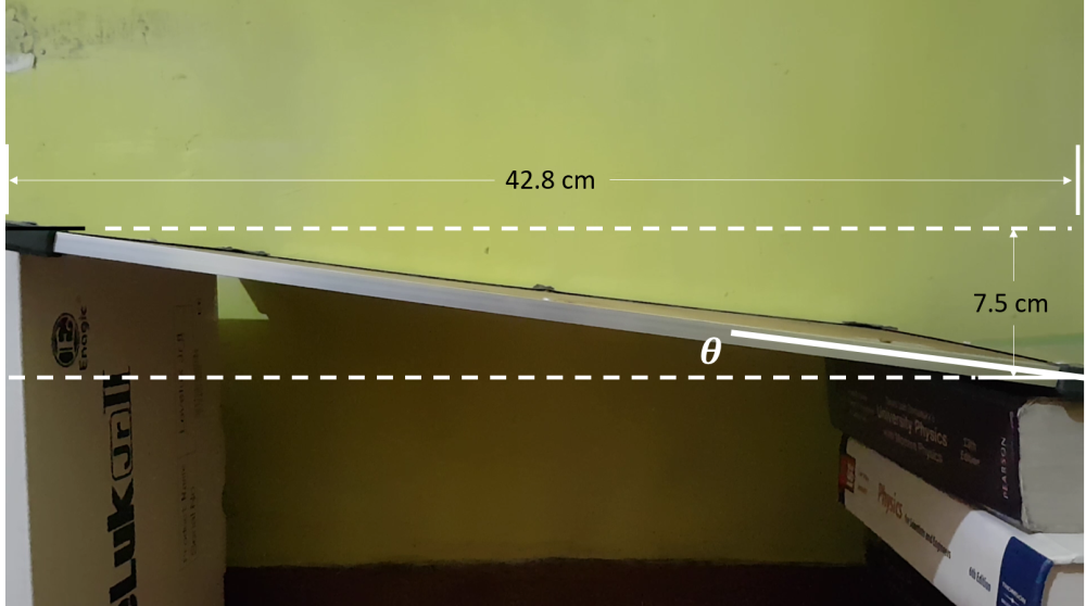
I used my mini white board as the incline, and fortunately I was able to find a golf ball among my old stuff. I did not have a camera and a tripod, so I used a smart phone with a ring accessory for its stand. I finally made use of my old physics books as a way to elevate the white board and the camera (just joking!). Here is a picture of the setup:

Fig 1. Kinematics experiment setup with measurements

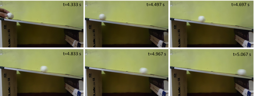
Upon recording the video, we would want to get the individual frames relevant to our experiment. I downloaded VirtualDub and loaded my video file. Each digital video has a frame rate or fps that tells you the time interval between consecutive frames as 1/fps. According to VirtualDub, my video has an fps of 30 Hz, so the frames are spaced at 1/30 or 0.033 seconds. I selected the the relevant interval for which the ball started to roll down the incline up until it reached the bottom. After exporting, I ended up with 23 frames exclusive of the time interval  4.3 seconds to 5.1 seconds. Here’s a sample of the frames I extracted from the video:

Fig 2. Sample frames indicating their time according to the original video.

II. Image Segmentation and Data collection

After obtaining our images, we are now set to segment the moving object in our video to collect the time varying variables in our kinematic experiment. We need to isolate the golf ball in our images and calculate its centroid to track its position through time. My first step was to try color segmentation, however I was unsure whether parametric or non-parametric segmentation would work better. I tried both, and here are the results:

Fig 3. Color segmentation of Frame 0 using a) parametric segmentation with threshold of 0.1, and b) non parametric segmentation with bin size of 64

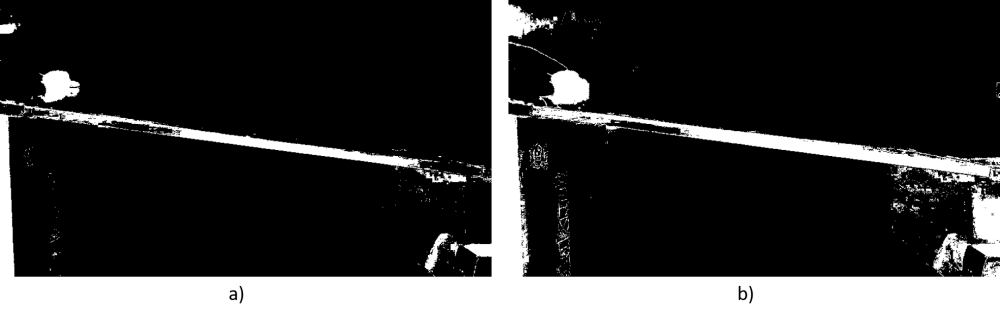
From the results above, we can see that parametric color segmentation was able to reduce the amount of unnecessary information in the result compared to the result of the non-parametric result. However, I opted to use the non-parametric approach since what is important is the object of interest, which is the golf ball. It was able to capture the shape of the object more accurately compared to the parametric approach, which will provide more reliable results in the long run.

Now that we have a preliminary result of image segmentation, we can further clean our subject image by using morphological operations to remove the other image elements. Obviously, a circular structuring element was appropriate for this image, however I used trial and error to get the suitable size to isolate the ball:

Fig 4. Comparison of the results after using the opening operator with a structuring element of different radius.

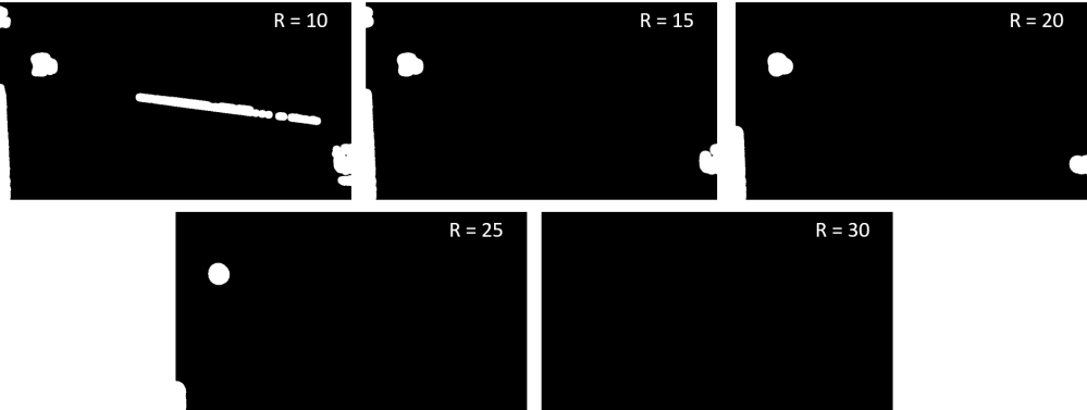
It can be seen that as the radius of the circular structuring element was increased, the amount of remaining elements were reduced, with a radius of 30 completely removing everything. From here, I saw that a radius of 25 would be appropriate, with the added benefit that the remaining blob was transformed into a more circular shape.

The next step would be to remove the remaining image elements aside from the ball. My approach for this was to generate an area histogram for each image to find out the range of areas of the ball and the other blobs. Afterwards, I filtered the blobs based on the area that I was able to get for the ball. This worked well for a few frames, until some blobs would appear to have areas that overlapped with the initial area range of the ball. I also thought that the ball would have the largest area among the remaining blobs, allowing me to set a minimum area size as a filter however still some blobs would defy my ideas. After a few minutes of brainstorming..

… I thought that since there is only a certain range of locations where the ball will appear, I had an idea of using a hard filter to block out all other pixels outside of this range. I used MS Paint to see the the maximum and minimum limits of the vertical location of the ball, and it was a success! I looked at each frame and only the ball was left each time.

The next step was to obtain the location of the ball at each frame, and we can do this by calculating the centroid of the ball bob. If you can’t recall, the centroid is the average location of the blob based on the involved pixels. So we need to calculate the x and y locations of each pixel in the ball blob and compute their mean. After setting up the code, we can now loop through all of the frames to calculate their centroids! However, due to the color segmentation section and the number of frames, it took a while to finish..

II. Data Analysis

After collecting our centroid data, we can now analyze it to calculate the acceleration due to gravity g. Now it’s time to do some basic calculations first. Let’s look at the free-body diagram of our setup:

Fig 5. Free-body diagram of the experiment

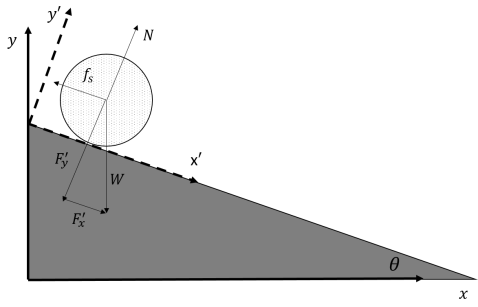
I used a rotated axis denoted by the ‘ to calculate the motion along the inclined plane. This would make it easier compared to using the original cartesian coordinates. With the ball ball having mass m, we have the following equations:

Where  is the normal force exerted by the incline on the ball, is the weight of the ball, and is the frictional force on the ball. Given these equations, we can calculate the acceleration of the ball along the incline to be

We don’t know the value of the frictional coefficient so we’ll leave this for later. To measure the acceleration of the ball in the video, we can use the kinematic equations of motion to find a relation between the displacement along the incline s against the time t:

Where is the effective acceleration of the ball. If we set the centroid of the ball at the top of the incline as the $s = 0$ then we can plot its displacement for each succeeding frame and use linear regression to get the slope.

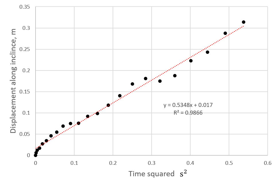
Fig 6. Plot of the displacement along the incline against with a linear regression fit.

Fig 6 shows the plot of the obtained displacement values along the incline with respect to the ball’s initial position. There are some oscillation of the values in the y-axis, however I suspect that it is due to the color segmentation results wherein the light reflecting from the ball varies with its position. Despite this, we were able to get a linear coefficient value of 0.9866, which is reasonable enough. From our previous equation, the slope is equal to half of the effective acceleration, so our measured value for the effective acceleration is .

Upon going back to our previous calculation of the effective acceleration, I realized that there are some things that I was not able to consider in doing those calculations. I treated the ball as a point mass (which is usually done in physics problems), when it definitely is not, as it has a finite radius r = 2 cm. This should definitely be accounted for especially since the ball is rolling along the incline instead of slipping. So I decided to redo the calculations, applying Newton’s Second law for Rotation:

Using the non-slip condition for acceleration [1], we can now solve :

For a solid ball of mass m and radius R, the moment of inertia is given by . With this, our effective acceleration is

Whew! With this new equation, we don’t have to know the friction coefficient, and we don’t even need to measure the mass and radius of the ball! Based from our measurements, our incline has an angle of with respect to the horizontal. This amounts to a value of with a percent error of 10.8%. It’s not actually big, but it’s quite significant, unfortunately.

After thinking about this activity, I realized that there are some factors that may have contributed to the discrepancy in the result. The first is the segmentation process, which I suggested earlier. Due to the motion of the ball, its image is blurred in the video, which could have contributed to unwanted translations of the centroid. The ball may have also experienced some tiny bumps that caused it to jump slightly during its rolling motion. Lastly, there was a problem with using the reference length in the video. Due to the perspective of the camera, the side closest to the camera is longer than the other parts of the board parallel to it. So when I placed the ball on the board, its centroid is at a different position compared to the edge of the board. Thus, the displacement of the centroid will be shorter than the actual board, which may have contributed largely to the measured effective acceleration.

IV. Conclusion

Despite the mishaps, I think that we were able to grasp the idea of video processing. Overall, this is actually a very fulfilling activity, as I was able to play around with a new concept (video) while applying some of the things I learned during this semester as well as some lessons in basic physics. This activity opens up more possibilities of doing things, such as physics experiments, and I am very thankful to Ma’am Jing for giving as the opportunity to learn and strive. I would rate my work with a score of 11/10 since I was able to follow the necessary steps in achieving my goal, however there is still room for improvement in terms of technicalities and such.

Reference

[1] Tipler, P., Mosca, G., “Physics for Scientists and Engineers”, 5th ed, W. H. Freeman and Company, 2004, pp. 288-291.